| x | y | color |
|---|---|---|
| 7.8 | 6.1 | blue |
| 13.7 | 4.5 | red |
| 21.0 | 5.7 | blue |
| 24.6 | 14.8 | blue |
| 18.9 | 21.8 | red |
| 5.0 | 14.8 | red |
| 13.4 | 17.1 | red |
| 32.3 | 2.8 | blue |
| 34.9 | 20.3 | blue |
| 32.6 | 12.3 | red |
Decision Trees
Reddy Lee
2024-03-08
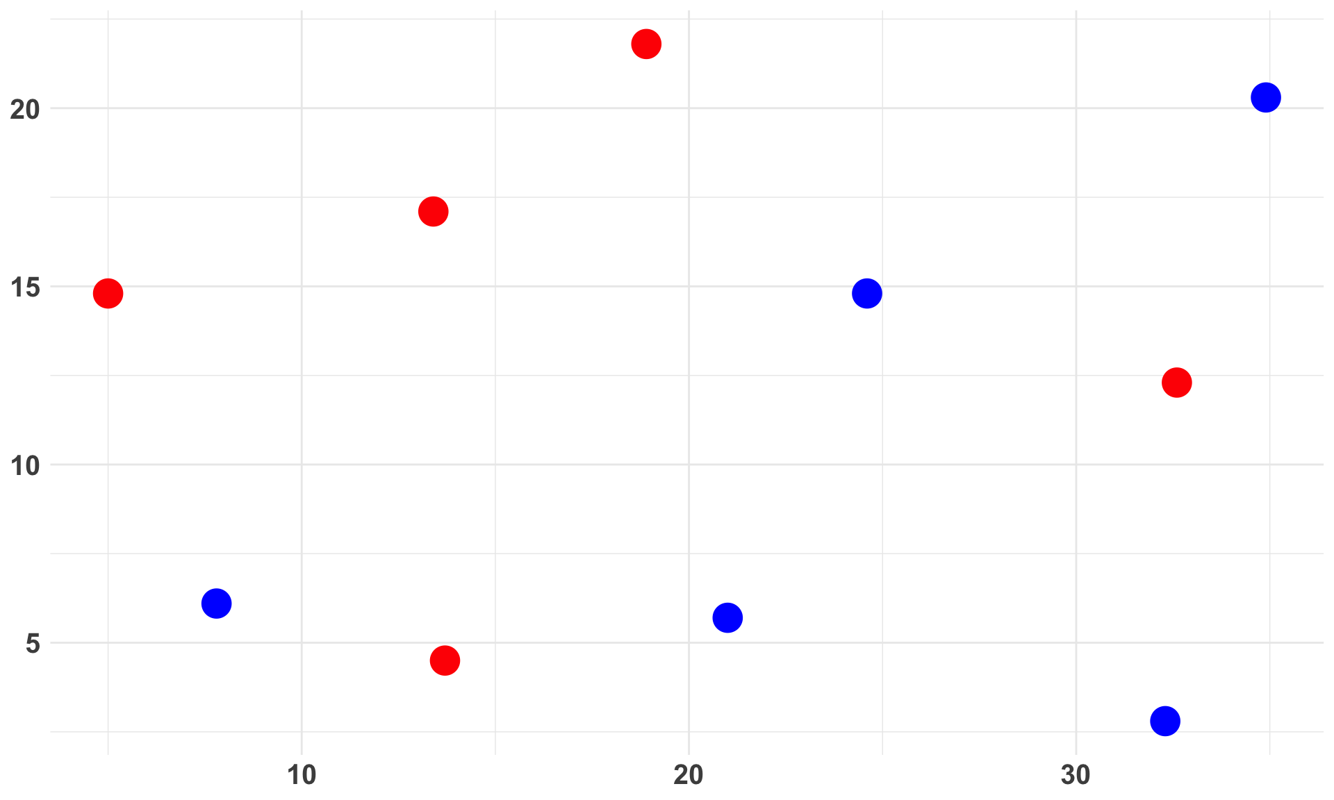
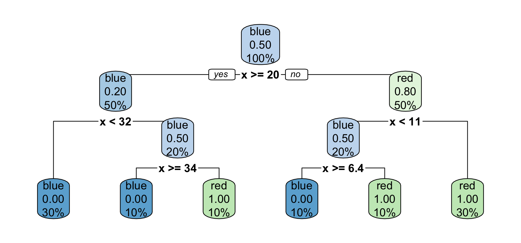
In this vid, we’ll manually construct a decision tree classifier using the following data set.
Decision trees
A decision tree classifier applies a divide-and-conquer algorithm to the training set, recursively splitting it into pieces that are as homogeneous as possible.
Here’s how I made that plot:

Can.Do.So • 耕读社


